
Correlation

What is correlation?
Correlation is a measure of the strength and direction of the linear relationship between two investments—that is, how they tend to perform relative to one another across time. The concept is relatively simple, but frequently misunderstood.
Generally speaking, if two investments are positively correlated, they tend to either underperform or over-perform together. That is, if Asset A and Asset B are strongly positively correlated, when Asset A over-performs relative to its expected return, Asset B tends to do the same. If Asset A and Asset B are negatively correlated, than the opposite is true. That is, when Asset A over-performs relative to its expected return, Asset B tends to underperform.
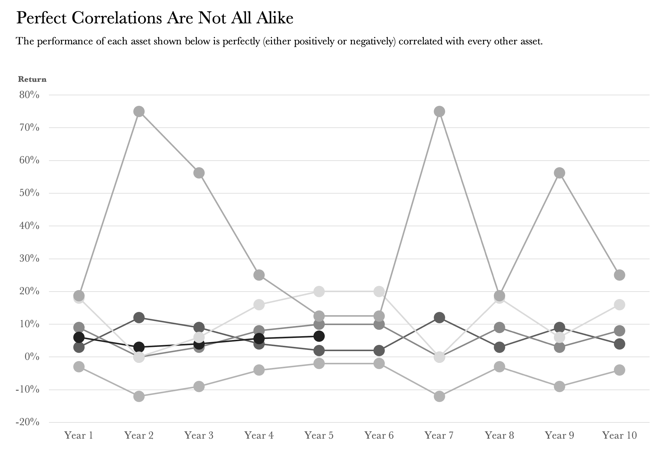
It’s commonly understood that a perfect positive (negative) correlation means that when the value of Asset A increases (falls), the value of Asset B increases (increases). But this isn’t necessarily true. Here’s an example of two assets that exhibit a perfect negative correlation. Note, there are no negative returns!
Asset A: 3%, 4%, 9%, 0%, 10%, 12%
Asset B: 9%, 8%, 3%, 12%, 2%, 0%
Correlation: - 1
How is it measured?
The strength of this relationship is measured by the Pearson correlation coefficient, which is a number on a scale ranging from negative one to positive one (-1 to +1). A coefficient of +1 denotes a perfect positive correlation, a coefficient of -1 denotes a perfect negative correlation, and a coefficient of 0 indicates the absence of a linear relationship.
Perfect linear relationships between different underlying assets don’t exist in the real world—correlation always falls somewhere between the two extremes (-1 and +1). For example, stocks and investment grade bonds in the U.S. have exhibited a correlation of approximately -0.20 over the past decade or so.
Why is it important?
Correlation lies at the heart of diversification. Imagine a portfolio holding ten different investments. At first glance, the portfolio might seem diversified. But if these investments are all highly positively correlated (i.e., they tend to over-perform or underperform at the same time), then perhaps the portfolio isn’t very diversified after all. If one investment underperforms, you can expect the rest to do the same. In theory, a portfolio comprised of uncorrelated or negatively correlated assets improves diversification and mitigates portfolio volatility over time.
How is it calculated?
Correlation between asset classes is calculated by reviewing how the assets tended to behave relative to one another historically. Of course, the real value lies in determining future correlation—there’s no guarantee that history will repeat itself. We arrived at the default correlation coefficients you see in Honest Math through a variety of sources on Wall Street and in academia, and we update our assumptions periodically.
Limitations of correlation analysis
Correlation specifically measures the linear relationship between two variables. It’s possible that two assets with little to no correlation could have a very strong non-linear relationship. In other words, there might be a relationship between the two assets, but it can’t be captured with simple correlation analysis.
Correlation is also prone to misinterpretation. You’ve probably heard “correlation does not imply causation”—a common refrain intended to remind folks to be wary of spurious relationships between variables. People have a natural inclination to find patterns in data, even if they’re meaningless, which makes us especially vulnerable to being fooled by randomness.
Moreover, correlation analysis also has a habit of failing us when we need it the most, which is during very volatile markets. In times of intense market turmoil, stocks across industries and countries often exhibit increased positive correlation regardless of their historical relationships. Sometimes it works the other way—asset classes with historically positive correlations can suddenly start moving in opposite directions. In early 2020, as markets tried to make sense of the COVID-19 pandemic, U.S. Treasury bonds and municipal bonds—two asset classes that have traditionally exhibited a strong positive correlation—started sharply moving in opposite directions. That is, tax-exempt bond prices moved sharply lower (yields increased) while taxable bond prices moved sharply higher (yields decreased), as if no fundamental relationship existed between the two types of investments. This (relatively) short-lived phenomenon was the result of a panic-driven “flight-to-quality”. That is, highly uncertain environments cause investors to move their money en masse to only the safest investments (U.S. Treasuries, in this case), resulting in unusual market distortions.